Trilinear fluorescence spectroscopy

Mikael Kubista, Jahan Ghasemi, Björn Sjögreen and Amin Forootan

MultiD Analyses AB, Göteborg, Sweden. E-mail: [email protected]

Introduction

Trilinear fluorescence spectroscopy is emerging as one of the most powerful techniques to study chemical equilibria, monitor chemical reactions and to analyse test samples. But what is trilinear fluorescence spectroscopy?

In traditional fluorescence spectroscopy, we measure excitation spectra, I(l_ex), emission spectra, I(l_em), or fluorescence intensity as a function of a physical variable that changes as the concentrations of the molecules present changes. We can, for example, measure spectra at varying pH, I(pH), temperature, I(T  ), or time, I(T  ). In trilinear fluorescence, intensity is measured instead as a function of three variables. Typically, these are the two wavelengths in combination with a variable, we can call a, which changes with changes in the concentrations of the fluorescent molecules:

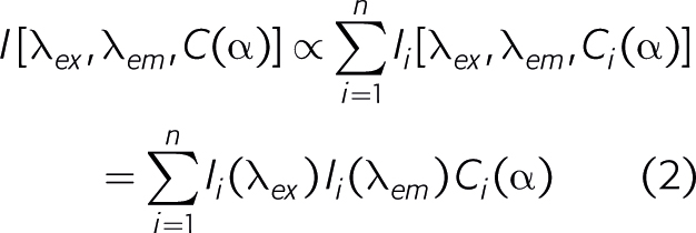
                I = I[l_ex , l_em , C(a)]         (1)

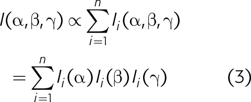
At low concentrations, the fluorescence of a mixture is the sum of the fluorescence contributions from the molecules present. Further, the fluorescence contribution from each pure molecular species can be written as a product of its concentration times its excitation intensity times its emission intensity:

The beauty of trilinear fluorescence is that the contributions from the different fluorescent molecules present can be determined solely from the measured data. No non-trivial assumptions are made and no auxiliary information about spectral shapes and concentrations is needed. Knowing I[l_ex , l_em , C(a)] one can calculate the emission spectra I_i (l_ex), the excitation spectra I_i (l_em), as well as the concentration profiles C_i(a) for all fluorescent molecules present by trilinear decomposition.^1,2 The principle of trilinear decomposition is illustrated in Figure 1. In essence, the trilinear measurement generates a cube of data, in which each data point is the intensity observed at the values of the variables indicated on the three axes. The proper name for the cube of data is three-way data.² Three-way data cannot be plotted in a single conventional graph, since four-dimensions are needed to plot intensity as a function of three variables. If the three-way data are trilinear, they can be written as a sum of the outer products of three vectors. Each term in the summation is the contribution from one fluorescent molecule, and the three vectors represent its intensities as a function of each of the three variables. Mathematically, it is possible to calculate all these vectors from the measured trilinear data set.² This is not possible starting with data sets of lower dimensionality. Unconstrained analysis of any two-way data, such as ex/em scans, I(l_ex , l_em), or spectral titrations, I[l, C(a)], yields results that are ambiguous due to linear dependence among possible mathematical solutions, which leads to degeneracy.³ This degeneracy disappears when the number of measurement variables is three or more. Below we show some applications of trilinear fluorescence spectroscopy analysed using DATAN. The data in the examples as well as the DATAN software are on www.multid.se.

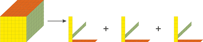
Figure 1. Graphical illustration of trilinear decomposition

DNA–ligand interactions

Binding of ligands to proteins and nucleic acids is of immense interest because of its biological relevance. Spectroscopic methods are very popular for characterising these kinds of interactions. Yet, most experiments are still performed as single-point measurements and data are analysed with very constrained models such as Scatchard, Hill and McGhee Von Hipple plots.⁴ If at least one out of the ligand and the target is fluorescent, trilinear fluorescence spectroscopy is the method of choice to study these interactions. Figure 2 shows an example. The dye thiazole orange was mixed with the nucleic acid polymer poly(dG) at a ratio of one dye molecule bound either per 80 (Figure 2, left panels) or per 40 (Figure 2, right panels) bases, and the two samples were characterised by trilinear fluorescence spectroscopy. As a self-consistent test, two independent characterisations were made. In one characterisation, emission spectra were measured at a number of excitation wavelengths (Figure 2, top) and in the other excitation spectra were measured at different emission wavelengths (Figure 2, bottom). The trilinear system is I(l_ex , l_em , r), where r is the dye/base binding ratio. If the concentrations of bound species depend on binding ratio, we have: I[l_ex , l_em , C(r)]. The two pairs of ex/em scans were decomposed independently by trilinear decomposition. The results are shown in Figure 3. Top graphs are calculated from the emission scans and the bottom graphs are calculated from the excitation scans. When comparing the plots, note that the wavelength intervals on the x-axis are slightly different. Clearly, the two decompositions agree very well and are evidence of the successful analysis. Both reveal the presence of two fluorescent species. Since unbound thiazole orange has no fluorescence, there must be two bound species. From the calculated spectra they are recognised as bound monomer and bound dimer.⁵ The trilinear decomposition also determines the relative concentrations of the two species. At low binding ratio (one dye per 80 bases) 80% of the dye binds as monomer, while at high binding ratio (one dye per 40 bases) 60% is bound as dimer.

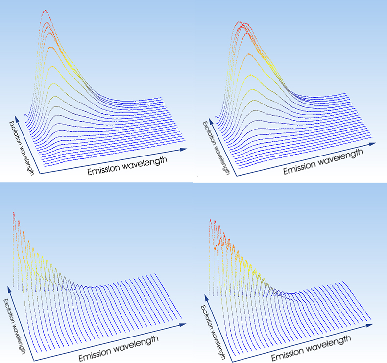
Figure 2. Ex/em scans of thiazole orange bound to poly(dG). Top graphs show emission spectra measured at different excitation wavelengths and bottom graphs show excitation spectra measured at different emission wavelengths. In the left graphs one dye is bound per 80 bases and in the right graphs one dye is bound per 40 bases.

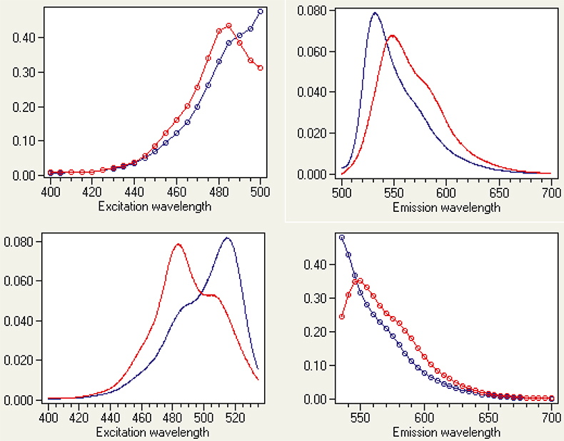
Figure 3. Calculated excitation and emission responses of two bound thiazole orange species. Responses in the top panels are calculated from the scanned emission spectra, and responses in the bottom panels are calculated from the scanned excitation spectra. Note that analysis of the set with scanned emission spectra produces continuous emission responses and discrete excitation intensities and, vice versa, i.e. analysis of the set with scanned excitation spectra produces continuous excitation intensities and discrete emissions

Chemical equilibrium

Trilinear fluorescence spectroscopy is a most powerful technique for studying chemical equilibria. Because of the very large amount of data typically collected in trilinear spectroscopy, equilibrium constants are determined with excellent accuracy. This is the case even when the titration end-points are not reached. As example, we determine the pKa between the fluorescein mono and dianion by ex/em pH titration. Ex/em scans were measured in the emission interval 470–650 nm using 390, 400, 410, 420, 430, 440, 450 and 460 nm excitations at different pH in the interval 5.66 £ pH £ 8.30 (Figure 4). Presence of two protolytic species was established by statistical indicators,⁶ and the data were decomposed into components’ specific responses by trilinear decomposition (Figure 5). Measured and reconstructed spectra from the calculated component specific responses are compared overlaid in the top left graph. Reconstructed data are shown in green and the original spectra in magenta. Overlap is almost perfect. The calculated emission spectrum and excitation intensities of the fluorescein dianion are indistinguishable from those measured in 1 M NaOH, where the dianion is the only species present.⁷ The monoanion cannot be obtained in pure form and direct comparison of calculated and measured spectra is not possible. But the results are in excellent agreement with previous determinations of the fluorescein monoanion spectra.⁷ The calculated molar ratios reveal that the two fluorescein species have the same concentrations at pH = 6.41. Although we have assumed no model, this is the protolytic constant of fluorescein with two decimals precision.⁷

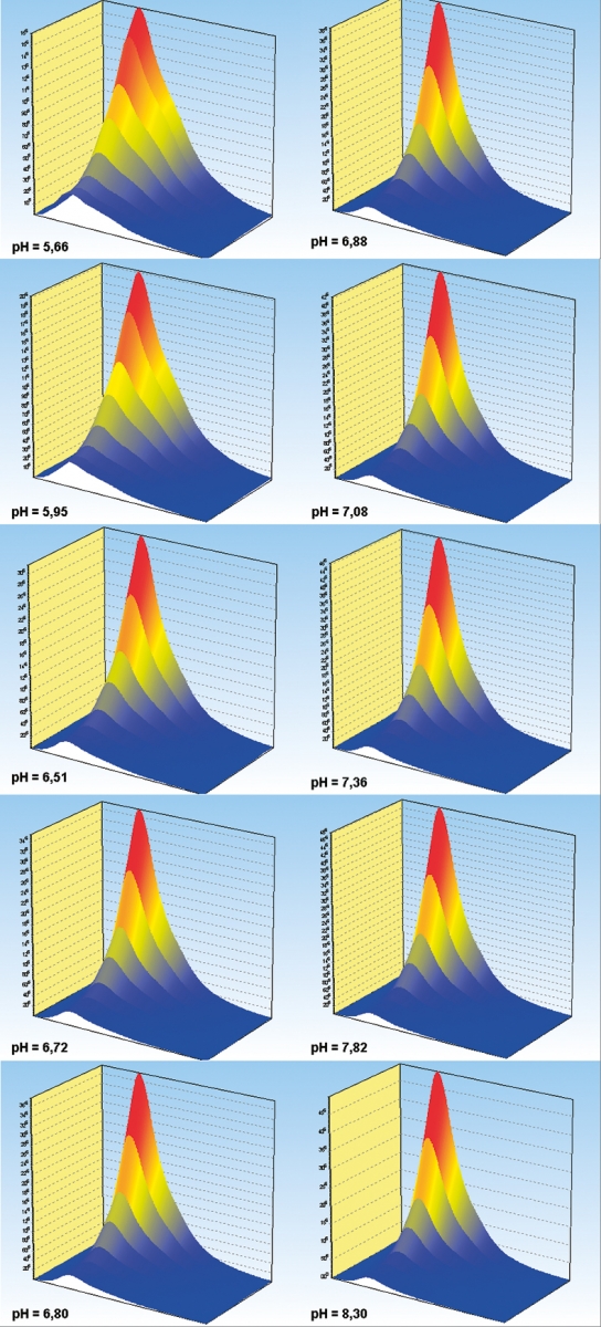
Figure 4. Emission spectra of fluorescein at pH = 5.66, 5.95, 6.51, 6.72, 6.80, 6.88, 7.08, 7.36, 7.82 and 8.30 measured between 470 and 650 nm using 390, 400, 410, 420, 430, 440, 450 and 460 nm excitation.

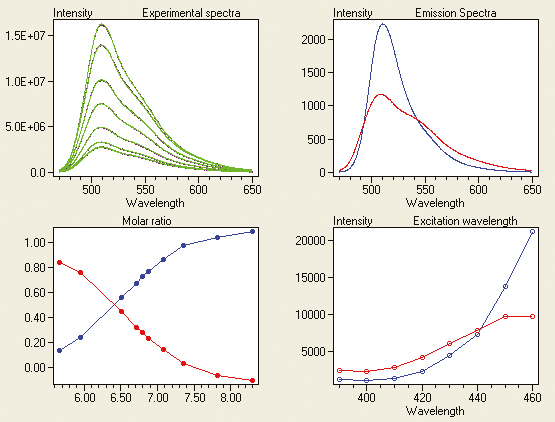
Figure 5. Results of trilinear decomposition of the fluorescein titration in Figure 4. Top-left graph compares overlaid measured (magenta) and reproduced (green) spectra at pH 5.66. Calculated emission responses are shown in the top-right panel, calculated excitation responses are shown in the bottom-right panel, and calculated molar ratios are shown in the bottom-left panel. Responses of the monoanion are shown in red and those of the dianion in blue. The lines in the graphs connect calculated data points and are only included to guide the eye.

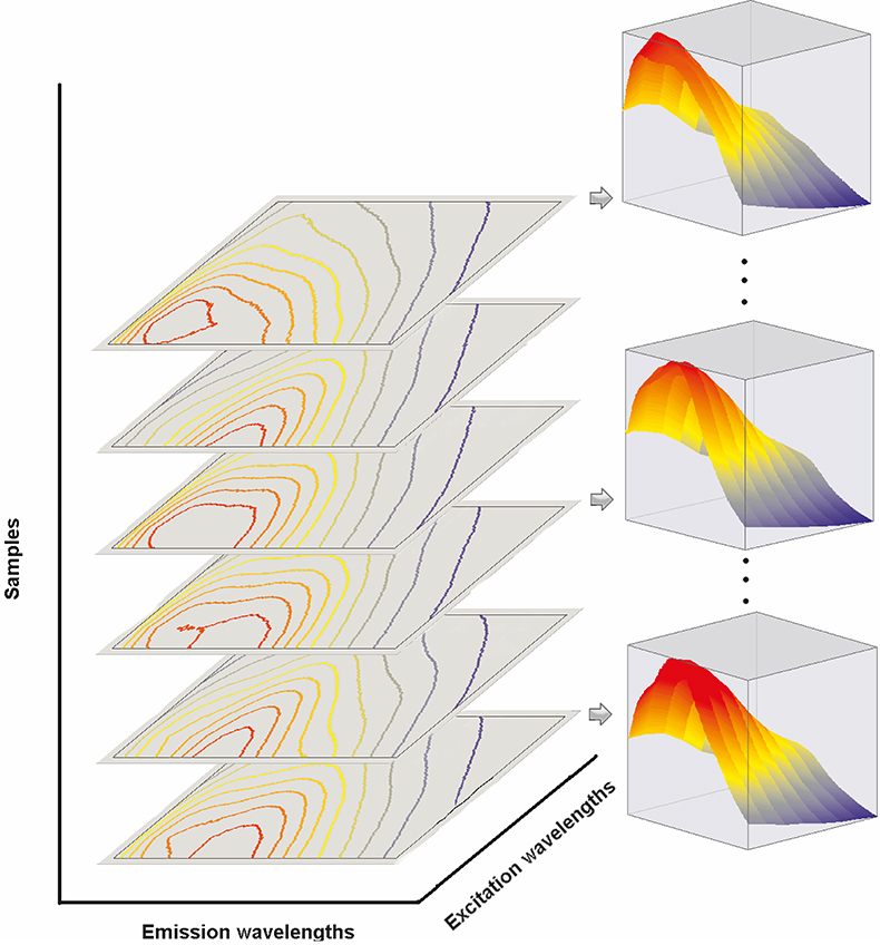
Figure 6. Six ex/em scans shown as contour plots of test samples containing Fluorescein, Eosin Y, Rhodamine 6G and Rhodamine B. Three are also shown as 2D-surface plots. The emission spectra were scanned between 500 and 600 nm using 460, 465, 470, 475, 480, 485, 490 and 495 nm excitations.

Independent test samples

In the examples above, equilibrium systems were studied. But trilinear fluorescence spectroscopy is not limited to studying interacting species. Any test samples that have common components can be analysed. Not all components have to be present in all samples, but each component must be present in at least two of them. Figure 6 shows contour plots of ex/em scans of six test samples containing different amounts of the four dyes Fluorescein, Eosin Y, Rhodamine 6G and Rhodamine B. For three of the samples the ex/em scans are also shown as 2D-surface plots. Statistical indicators revealed the presence of four distinct fluorescent species,⁶ and their fluorescence emission spectra and excitation responses were calculated by trilinear decomposition (Figure 7). Agreement between measured (magenta) and reproduced (green) spectra is excellent (Figure 7, top left), and both emission spectra and excitation responses are nicely resolved despite extensive spectral overlap. The relative concentrations of the components in the six test samples were also calculated, and found to be highly accurate by comparison with values determined from independent methods.

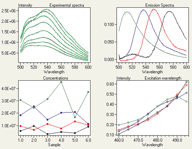
Figure 7. Calculated spectra and concentrations of Fluorescein, Eosin Y, Rhodamine 6G and Rhodamine B by trilinear decomposition of the ex/em scans of the samples in Figure 6.

Limits and possibilities

Trilinear fluorescence spectroscopy opens up new possibilities to characterise test samples, and to study chemical equilibria and chemical reactions. The criterion for successful trilinear analysis is that intensity is measured as a function of three variables that affect the fluorescence independently:

At low concentrations, the excitation spectrum of pure fluorophores is usually independent of emission wavelength, and the emission spectrum is independent of excitation wavelength (the Kasha–Vavilov rule). Also, the intensity contribution from each fluorophore is proportional to its concentrations. This leads to:

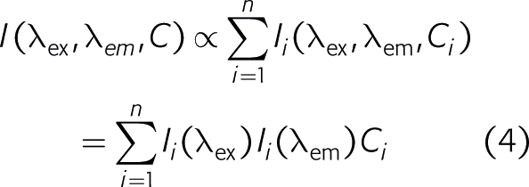
which is the required criterion for trilinear analysis. If the fluorophores interact through energy transfer Equation (4) is violated. Likewise, if the concentration of one fluorophore is proportional to that of another fluorophore their contributions cannot be separated.⁸ Hence, series of samples for trilinear analysis cannot be created by a simple dilution of a test sample, because dilution normally does not change the relative concentrations of the different chemicals. However, extraction does, and is indeed an excellent procedure to create sample series for trilinear fluorescence analysis.⁹ Time is an excellent variable in trilinear fluorescence spectroscopy. It can be reaction time of a chemical process or decay time after light excitation, or even both. The beauty of time-resolved trilinear fluorescence is that spectral responses of intermediate species can be determined even if the species are present neither at the start nor at the end of the reaction.¹ Another interesting variable is the polarisation of light, which distinguishes the fluorophores by their rotational diffusion times. When combined with ex/em scans the spectral responses of fluorophores in a single sample can be separated.¹⁰

In summary, trilinear fluorescence is possibly the most powerful spectroscopic method to analyse sample mixtures. Without any auxiliary information the spectral properties and concentrations of the components are determined. The only requirements are that the spectral responses of the components are linearly independent and that the relative concentrations of the components vary among the samples.

References

1. M. Kubista, Chemometr. Intell. Lab. Syst. 7, 273–279 (1990)
2. Smilde, R. Bro and P. Geladi, MultiWay Analysis. John Wiley & Sons, ISBN 0-471-98691-7 (2004).
3. W.H. Lawton and E.A. Sylvestre, Technometrics 13, 617–633 (1971). https://doi.org/10.1080/00401706.1971.10488823
4. V.A. Bloomfield, D.M. Crothers and I. Tinoco, Nucleic Acids Structures, Properties and Functions. University Science Books, Sausalito, CA (2000).
5. J. Nygren, N. Svanvik and M. Kubista. Biopolymers 46, 39–51 (1998). https://doi.org/10.1002/(SICI)1097-0282(199807)46:1<39::AID-BIP4>3.0.CO;2-Z
6. Elbergali, J. Nygren and M. Kubista, Anal. Chim. Acta 379, 143–158 (1999).
7. R. Sjöback, J. Nygren and M. Kubista, Spetrochim. Acta A 51, L7–L21 (1995).
8. Scarminio and M. Kubista, Anal. Chem. 65, 409–418 (1993).
9. Nygren, A. Elbergali and M. Kubista, Anal. Chem. 70, 4841–4846 (1998). https://doi.org/10.1021/ac980381n
10. M. Kubista, J. Nygren, A. Elbergali and R. Sjöback, Critical Rev. Anal. Chem. 29, 1–28 (1999). https://doi.org/10.1080/10408349891199275